introduction
The exome era turns five years old this fall, with the anniversary of the “Targeted capture and massively parallel sequencing of 12 human exomes” [Ng 2009]. Born at a time when whole genome sequencing cost about a quarter million dollars, exome sequencing provided the cost savings that made sequencing large numbers of individuals for research feasible. Here in the MacArthur lab, our rare disease gene discovery projects rely on whole exome sequencing (WES) as a first pass on unsolved Mendelian families. If we can’t find a causal variant, we perform WES on additional family members. If we run out of family members and still haven’t found a likely causal variant, only then do we turn to whole genome sequencing (WGS), often alongside functional analyses such as RNA sequencing from muscle tissue.
WGS has remained a last resort for a few reasons: it’s still a bit more expensive than WES, it produces more data we have to process and store, and despite some notable recent advances [Ritchie 2014, Kircher 2014] our ability to interpret the pathogenicity of variants in the 99% of the genome that doesn’t code for protein is still a far cry from what we can do with exons. But we still turn to WGS for two main reasons: (1) its superior ability to call structural variations by covering the breakpoints, and (2) its more reliable coverage of the exome itself.
We now have 11 individuals from Mendelian disease families on whom we’ve performed both standard WES and very, very high-quality WGS, which gives us a chance to quantify exactly what we’re missing in the WES. The question of what we’re missing in WES is one input to our periodic re-evaluation of whether WES is still the best value for research dollars or if we should be turning to WGS right away.
In this post, I’ll explore the “callability” of these 11 WES samples: how much of the targeted exome is covered at a depth where one could hope to call variants, and how many variants are missed, and why? We’ll should say up front that this isn’t a product comparison – the WGS on these samples is of much higher quality than is standard these days, and our exomes are comparatively out of date, so this post cannot directly inform the “WES vs. WGS” decision.
the data
We have 11 individuals from Mendelian muscle disease families on whom both WES and WGS were performed. Again, this is not designed to be a totally fair comparison, and the WES and WGS datasets differ on several dimensions:
|
WGS |
WES |
| Capture |
None |
Agilent SureSelect Exome |
| Amplification |
PCR-free |
PCR amplified |
| Read length |
2×250bp |
2×76bp |
| Mean depth |
30-90x |
80-100x |
Many of the limitations we see in our analysis below are not actually inherent in exome capture but rather relate to PCR amplification or read length. And here are a couple of other caveats: some of the samples were deliberately WGS sequenced at 30x coverage and others at 60x coverage, so the “platinum standard” to which we’re comparing the WES data is a bit of a moving target. Finally, we are only considering one rather outdated exome capture technology (Agilent SureSelect v2) and not a survey of available products; the Broad, for instance, has recently moved to a substantially better capture technology (Illumina’s ICE technology), which we now use as standard for our rare disease patients. We have been working on performing a fairer and more comprehensive comparison of WES and WGS, and the analysis in this post may be considered as a pilot analysis.
analytical approach
The code used for this analysis is here; in the post I’ll only present the results. Briefly, I analyzed (1) coverage depth, and (2) called variants.
For the coverage depth analysis, I used BEDtools to create four sets of genomic intervals:
Note that in this analysis I did not consider all Gencode intervals, as Agilent SureSelect does not even attempt to target some of these intervals. In exome sequencing, it goes without saying that you’re missing most of what you do not target; the question we want to address here is how much of what we do target we are still missing. (The question of relative coverage of all genic regions is a topic for a separate post.)
For each genomic interval, in WGS and WES, I then ran GATK DepthOfCoverage for every combination of minimum MAPQ of 0, 1, 10, or 20, and minimum base pair quality of 0, 1, 10 or 20. In other words, I computed the read depth across every base of these genomic intervals, stratified by mapping quality and by base pair quality.
For the called variant analysis, I used VCF files produced by GATK HaplotypeCaller. (An important caveat which I’ll repeat later is that the HaplotypeCaller calls were done in 2013 on a now-outdated GATK version and appear to contain a few bugs which may have since been fixed. When we repeat some of these analyses on a larger dataset we will use a newer callset.) I subsetted the variant calls to the Broad Exome and the samples of interest using GATK SelectVariants. I converted them to tables, decomposing multi-allelic sites into separate rows using GATK VariantsToTable, and then converting each allele to its minimal representation. The WES samples had been joint-called with a few hundred other samples, necessitating some further filtering at the analysis stage which I’ll describe below.
results
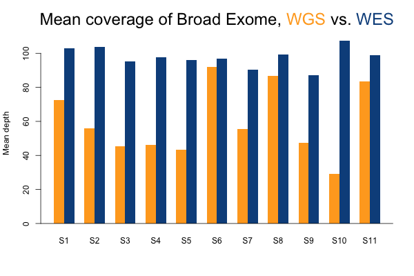
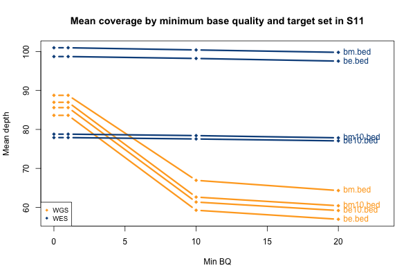
I’ll start with some descriptive statistics and then get gradually into the analysis. Although the samples were sequenced to a variety of mean exonic depths in both WES and WGS, it is categorically true across all 11 samples that the mean exonic depth of the WES data is higher than the WGS data:
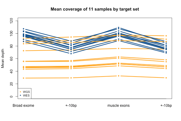
Again, recall that some WGS samples were sequenced with a goal of 30x coverage and others 60x, hence some of the variability in the height of the yellow bars. As you’d expect, the WGS BAMs have similar coverage in a 10bp buffer around all exons (or muscle exons) as they do in the exons themselves, while the WES has reduced coverage in the ± 10bp buffer regions. In the few samples with the deepest WGS sequencing (e.g. S11), WGS is actually deeper than WES in the buffer regions.
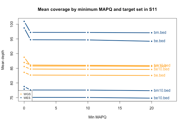
As mentioned above, I stratified the coverage calculations by minimum mapping quality of the read (MAPQ). The above plots are for all reads regardless of MAPQ. When I stratify by MAPQ, I find that just requiring MAPQ ≥ 1 loses you about 3% of your depth in WES and 2% of your depth in WGS. Being even stricter and requiring MAPQ ≥ 10 or 20 doesn’t lose you any depth at all. This is true regardless of the target set (the different lines, denoted at right). The below plot shows just sample S11 as an example, but the same is true across the 11 samples. A MAPQ of 0 indicates that the read’s alignment is ambiguous – it fits in more than one place in the genome. So the conclusion here is that a few percent of reads, in both WES and WGS, have MAPQ 0, but other than that, virtually all reads have a high MAPQ. This plot shows one sample, but they all look pretty similar to this:
The picture when stratifying by base quality (BQ) rather than MAPQ is only slightly more interesting, as seen below. Virtually all bases in the WES data have quality > 20, so quality thresholds up to 20 really have no hit on depth (flat blue lines). In the whole genomes, on the other hand, requiring base quality of 10 or 20 loses almost a third of the depth in the one sample shown here (yellow curves). Other samples were qualitatively similar though some of them were less dramatic. My suspicion is that this is not due to it being WGS per se, but rather the fact that 250 bp reads are near the limit of what next generation sequencing is presently capable of, so that getting such long reads involves some sacrifice in base pair quality at the ends of the read. Again, this plot shows one individual, but is typical of all of them:

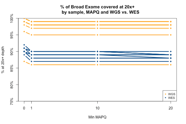
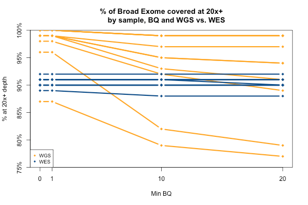
All of the above plots are concerning mean coverage across the entire target set. A different metric that might be more pertinent to callability is the percent of the target that is covered at 20x depth or better. Therefore I computed for each of the 11 samples what percent of the Broad Exome is covered at 20x or better, varying the minimum MAPQ threshold but applying no base quality cutoff. As the plot below shows, all but one of the WGS samples has > 95% of the exome covered at ≥ 20x when all reads are included, while the WES samples cluster closer to 90%. In both cases, you drop below the 20x threshold in about 1% of the exome by requiring that reads have MAPQ > 0. Requiring MAPQ of 10 or 20 doesn’t change things much.
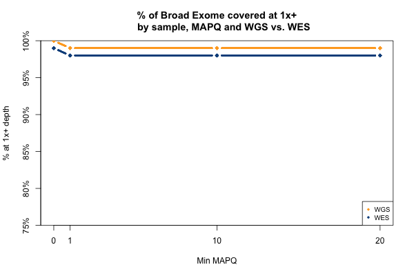
The picture is remarkably similar when the threshold you’re trying to achieve is 1x instead of 20x:
All 11 samples are plotted in blue and yellow above — you just can’t see them because they overlap perfectly. In all 11 WGS samples, 100% of the Broad Exome is covered with at least 1 read, but only 99% is covered with at least 1 read of MAPQ > 0. In all 11 WES samples, 99% of the Broad Exome is covered by one read, but only 98% by one read of MAPQ >0. Interpretation: about 1% of the exome is just utterly unmappable even with 250bp reads, and 2% is unmappable with 76bp reads.
The comparable picture 20x+ depth stratifying by base quality is more predictable: as above, the WGS but not WES samples here take a hit at the higher base quality cutoffs:
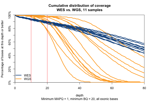
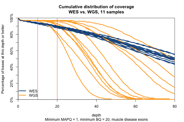
So far I’ve established that base quality only matters in my WGS samples, and MAPQ only differs between 0 and > 0. I’ve also established that these trends are pretty consistent across my different target sets. Therefore, I’m going to simplify and from here on out, I’ll only look at the Broad Exome, and I’ll either filter on MAPQ ≥ 1 and BQ ≥ 20, or I won’t filter at all. Fixing these variables lets us look more quantitatively at the distribution of coverage depth across the exome, instead of looking at mean coverage or at the percent covered at ≥ 20x. Here is a plot of the cumulative distribution function of depth in the 11 samples, in the exome, without any quality filters:
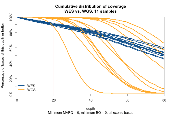
Remarkably, with just one exception, the WGS samples stay very close to 100% coverage up until about 20x depth, and then each at some point drops off sharply. The WES samples, in contrast, drop off very steadily. That’s bad. The ideal sequencing scheme would have every last base covered at exactly, say, 30x depth – enough to call any variant with high confidence – and then no bases covered at ≥ 31x depth – more isn’t useful. As expected, WGS is much closer to this ideal than WES. Phrased differently, WES has much higher variance of coverage. This is probably due chiefly to capture efficiency, and possibly to some extent due to GC bias during PCR amplification. This is why, even though our samples had much lower mean coverage in WGS than WES, the WGS provides us (with one exception) with a larger proportion of the exome covered at ≥ 20x.
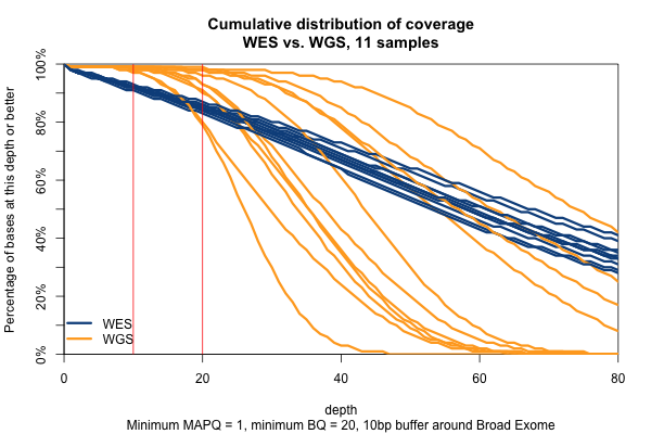
The picture is similar when we filter for MAPQ ≥ 1 and BQ ≥ 20 (below). The WGS coverage suffers a bit, particularly due to the base quality threshold, so that some of the WGS now have fewer bases at 20x coverage than WES. At 10x, though, WGS is still the clear winner.
With MAPQ > 0 and BQ ≥ 20, the WGS samples have an average of 98.4% of the exome covered at ≥ 10x, while WES only have 93.5%. So if you consider 10x the minimum to have decent odds of calling a variant, then the combination of longer reads (thus greater mappability) and more uniform coverage in these WGS samples is bringing an additional 5% of the exome into the callable zone.
Surprisingly, though we think of muscle disease genes as being enriched for unmappable repetitive regions, the above figure is nearly identical when only muscle disease gene exons are included. As expected, the advantage of WGS over WES is even clearer in the ±10bp around exons, though the shape of the curves is similar.
Moving on, let’s talk about variants called in the WES vs. WGS datasets. I decomposed the variant calls into separate alt alleles, so I’ll speak in terms of alleles rather than sites. This table provides a few descriptive statistics on alleles called when considering only the Broad exome with no buffer:
|
WES only |
WES and WGS |
WGS only |
| Alleles called |
5802 |
45372 |
2538 |
| PASS alleles called |
712 |
40078 |
2120 |
| of which at least one non-homref genotype has GQ > 20 |
451 |
|
2025 |
Although more alleles were unique to WES than to WGS, most of these were filtered variants. Moreover, even among the PASS variants in the WES set, many PASSed only because the WES samples had been joint-called with a few hundred other samples, while none of the 11 individuals considered here actually had an alternate allele call with GQ > 20. So basically, we have about 40,000 PASS alleles shared by both sets, 500 good-quality PASS alleles unique to WES and 2,000 unique to WGS. The Venn diagram for variants of decent quality looks something like this:
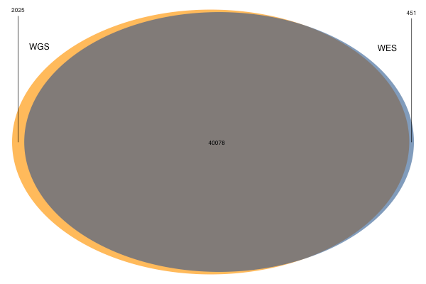
The figure for WGS is precisely in line with expectation: as shown above, WGS brings an additional ~5% of the exome up to a “callable” threshold, so it makes sense that it produces about 5% more alt allele calls.
As an aside, of the alleles called in both datasets, WES and WGS called the exact same genotype for all 11 individuals in 91% of alleles. At the other 9% of alleles, WGS had the greater alt allele count 67% of the time. This suggests that even when WES and WGS can both detect an allele’s existence, WGS may have greater power to call the allele in more samples.
Next I wanted to dig into the variant calls in a more anecdotal way. Which types of situations are better called by WGS and which are better called by WES? What are the error modes of each dataset? To get at this question, I looked at IGV screenshots of both the WES and WGS reads at sites where a variant was called in one dataset but not the other. I looked at all such discordant sites in muscle disease gene exons (16 sites), and then intended to look at a random sampling of 10 WES-only and 10 WGS-only alt alleles exome-wide, though I ended up doing this a few separate times as I tweaked the filters above. In the final run, with the PASS and genotype quality filters described above in place before the random sampling, I did not notice an obvious difference in the proportion of genotype calls that I concluded looked correct on IGV after viewing reads from both datasets. 6 of the 10 WES-only alleles looked like the correct genotype call had indeed been made based on WES, and symmetrically, 6 of the 10 WGS-only allele calls looked correct. Of the 40% that I didn’t deem exactly correct, most were suggestive of some sort of non-reference allele at the site, it just wasn’t exactly as called by HaplotypeCaller. The number of samples I looked at clearly isn’t enough to be getting into any more numbers, but this exercise was anecdotally very rich. I found it quite illuminating as to some of the error modes of genotype calling and the relative strengths and weaknesses of WGS and WES, and of long reads vs. short reads.
Based on all the screenshots I looked at, I would break the discordantly genotyped sites into 7 categories. What follows is a list of these categories, with one example for each, and a description of whether WGS or WES performed better and why. You can click the image to view at full resolution.
1. more consistent read depth without capture

Based on the coverage analysis above, which indicated that depth is much more variable in WES than WGS, I expected to see lots of these cases, and I did. Here there are only two reads in WES, and both happen to support a C>A SNP, so it was called in WES. My guess is that’s just bad luck – base errors happen in sequencing, and with only two reads, sometimes they’ll happen in the same spot on two reads. In WGS, there was much more depth and no read support for this SNP, so it wasn’t called.
I chose this example because it’s interesting to note that the variable depth in WES doesn’t just lead to missed genotypes, it also leads to false positives. As you’d expect, though, there were more cases where a real variant was called in WGS, and was missed in WES due to having only 0 or 1 or 2 reads. Here is one such example if you’re curious.
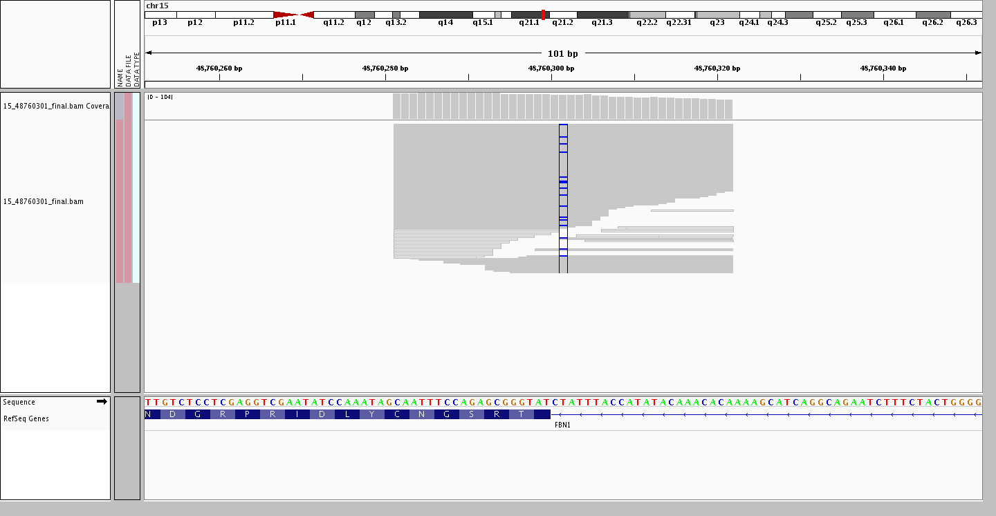
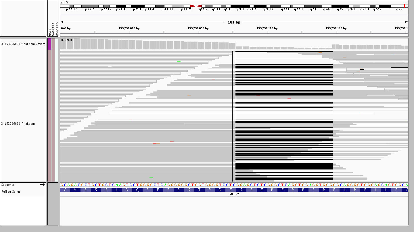
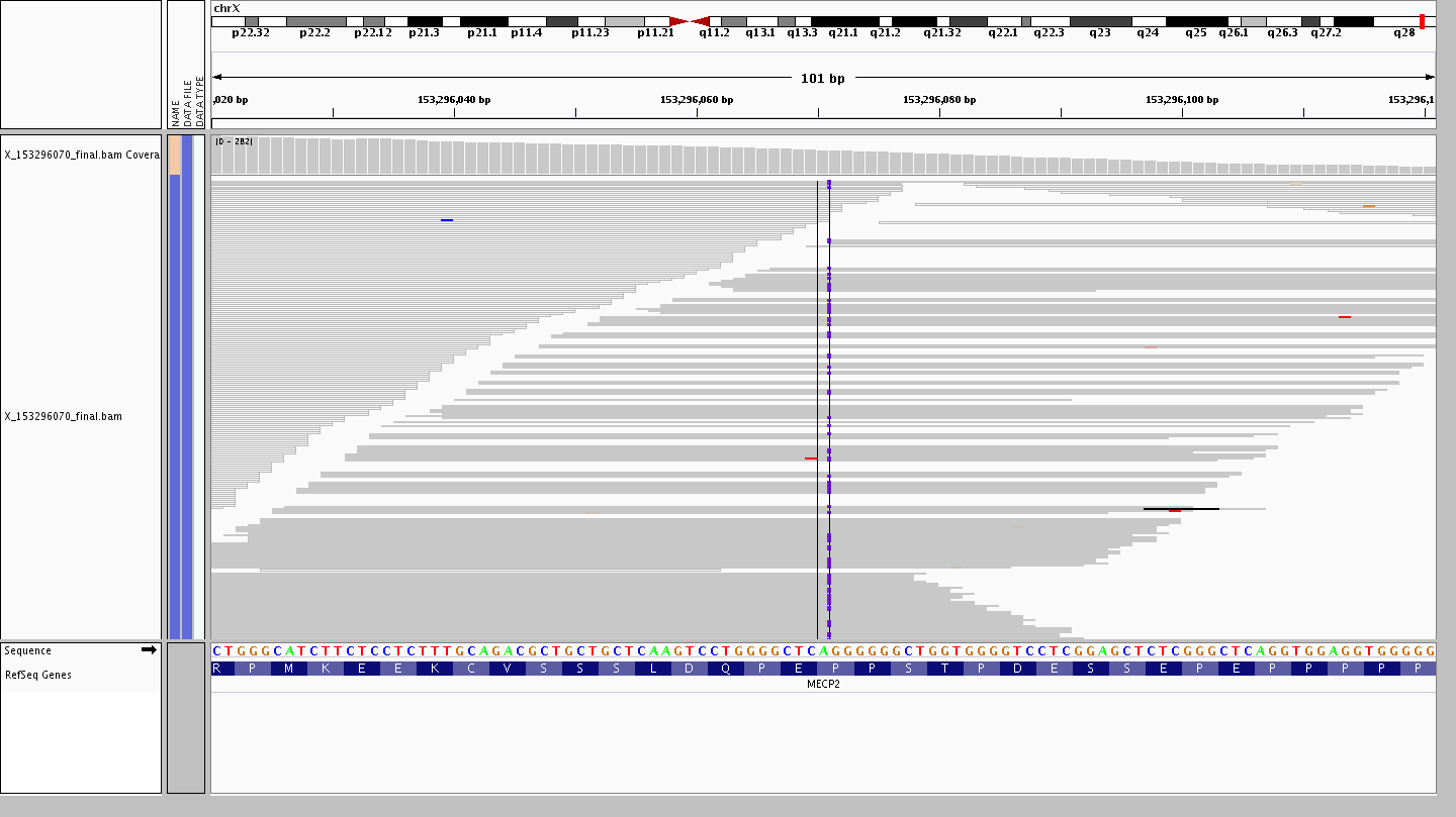
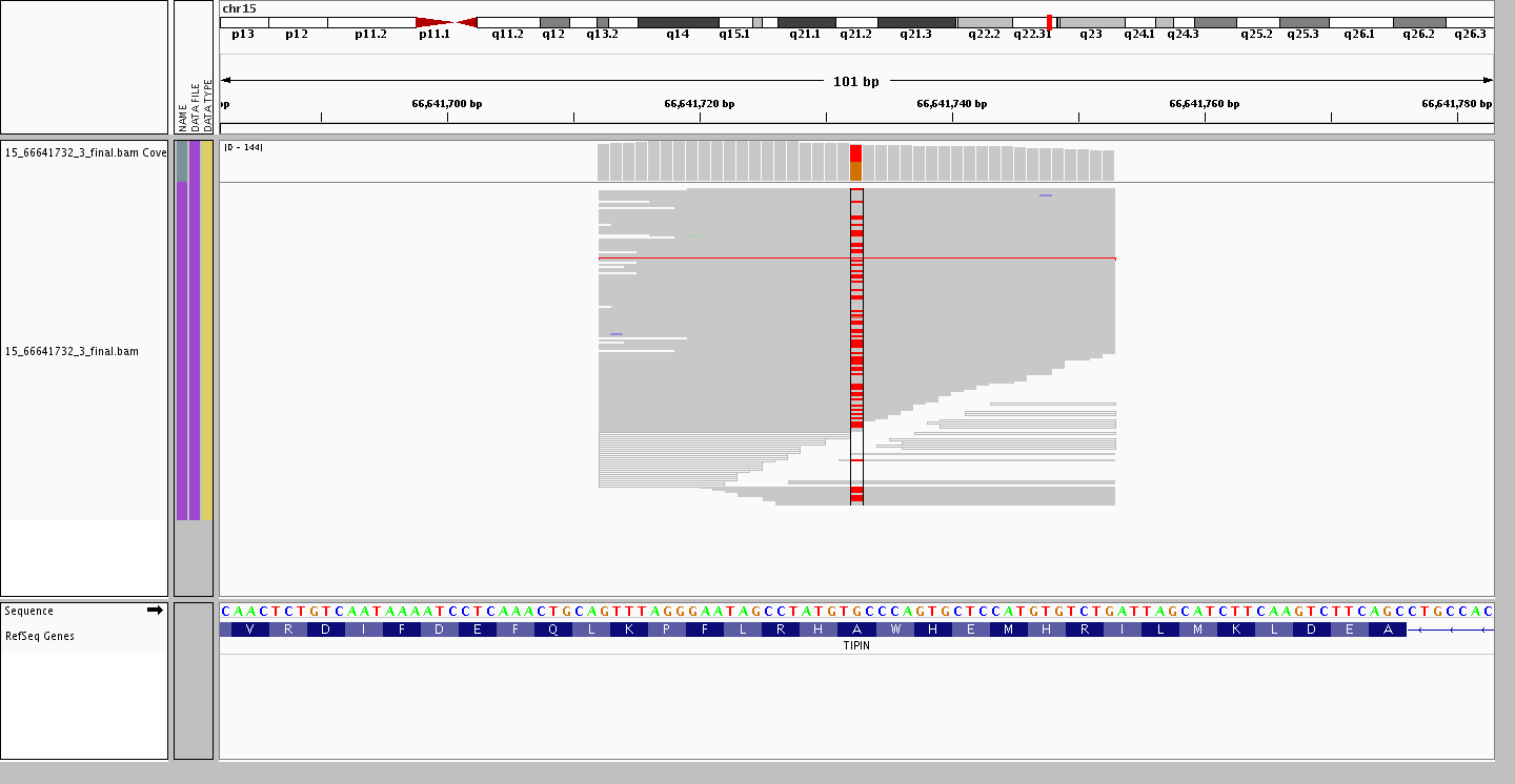
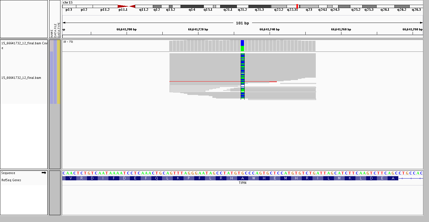
2. longer reads, better mapping quality

In WGS, this was called as a homozygous alt genotype. Most, but not all, reads support the alt allele; if you look closely, almost 100% of the gray (MAPQ > 0) reads do support the alt allele, while the ones that don’t are almost exclusively white (MAPQ of 0). In the WES, by contrast, there are no gray reads – all the reads here aligned with a MAPQ of 0. That’s because this region is similar enough to other regions that some (not all) 250bp reads can align uniquely, while no 76bp reads can align uniquely. Not only was this not seen as homozygous in the WES data, the variant wasn’t even called at all.
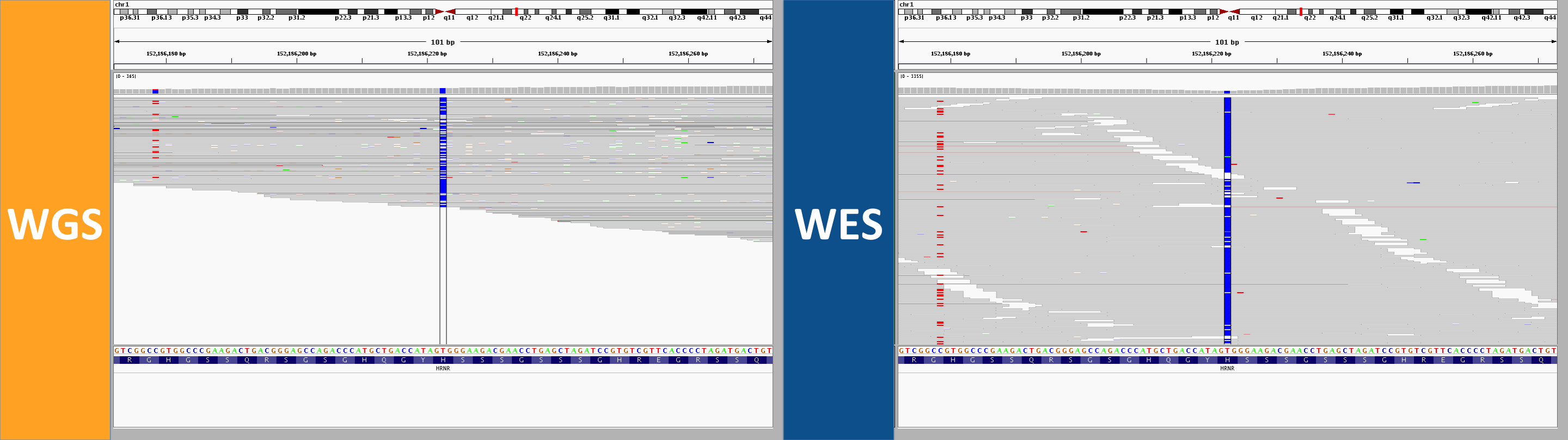
3. longer reads spanning short repeats

A different advantage of longer reads is their ability to span short tandem repeats or homopolymer runs. I looked at these screenshots because the WES data had called a 3bp in-frame deletion that was absent from the WGS calls. On very close inspection, here’s what happened. RRLLLF became RLLLLF – meaning that an R changed to an L, or an R was deleted and an L duplicated, however you prefer to think of it. The WGS data called a MNP in which tandem T>G and C>A mutations turned an R (TCG) into an L (GAG), a reasonable interpretation. In WES, almost half of reads supported that same interpretation, but a subset of reads (6 of them) failed to span the LLL repeat, so they didn’t see that there were 4 Ls instead of 3, and this resulted in a call of a 3-bp deletion of the R. If you look closely, two of these reads spanned into the F after the Ls, and had mismatched bases as a result. The longer reads in WGS, because they spanned the entire repeat region, gave the more correct call.
4. better distribution of position in read without capture

In these screenshots, a homopolymer run of As has contracted by 3 As compared to reference. In WGS, this was called as a left-aligned TAAA>T deletion, as it should be. In WES, no reads spanned the polyA tract, and so no variant was called. At first I thought this was just an issue of read length, but in fact, the polyA tract is plenty short enough to be spanned by 76bp reads in WES. My suspicion is that this relates more to capture. The capture probe for this exon in the Agilent baits file ends at the beginning of the polyA:
2 47641406 47641559 + target_20209
So perhaps it has captured fragments centered further left, such that only their tail ends protrude into the polyA area.
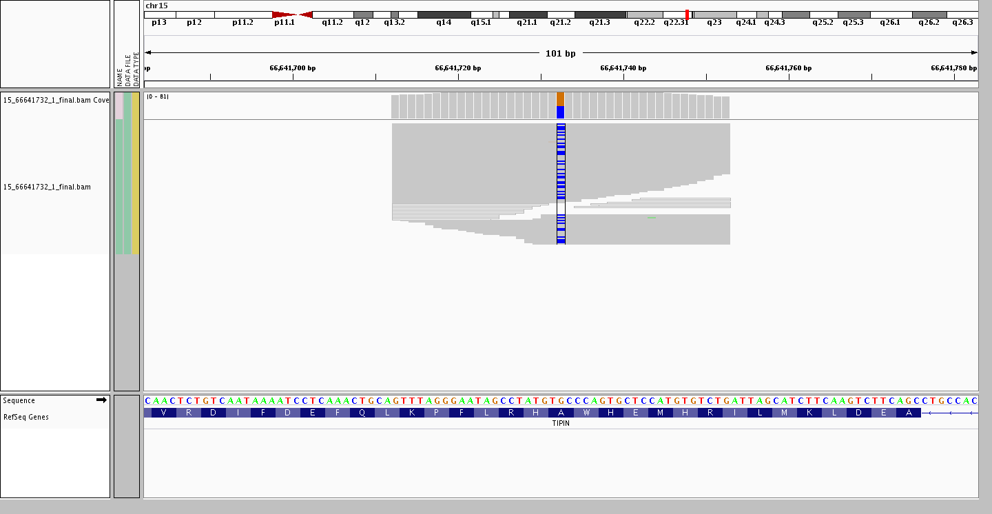
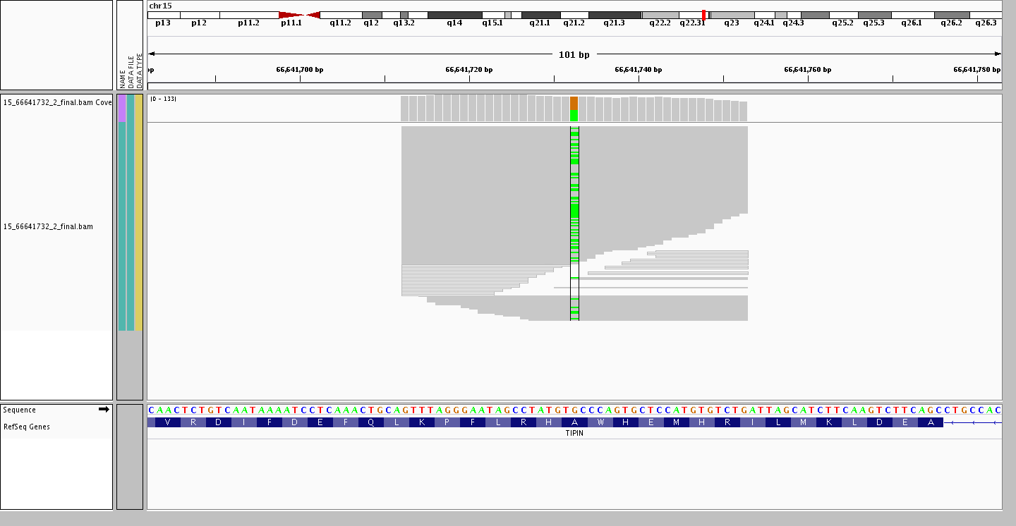
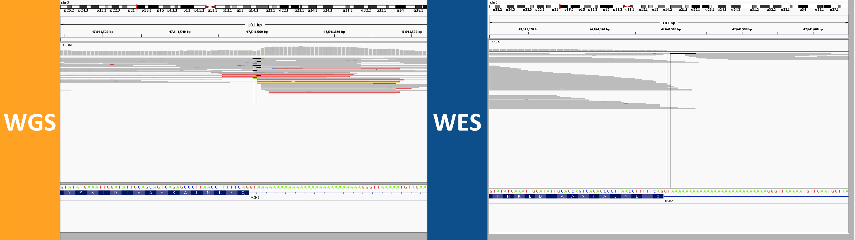
5. dense SNPs or MNPs interfering with capture

Although it appears intronic on the IGV track at bottom, this region is actually baited in the Agilent exome capture kit:
5 140186771 140189171 + target_50250
Thus making this a fair comparison. There are 7 non-ref bases in just a 12-bp stretch, making this a big MNP or a non-contiguous series of SNPs, depending on your perspective. They’re quite clearly all on the same haplotype. In WGS, they achieve about a 50% allelic balance, and were called as separate heterozygous SNPs. In WES, the allelic balance is way off, with only two alt reads. I see two possible explanations. The density of mismatches may be enough to throw off alignment of a 76bp read but not a 250bp read, or it may be that so many SNPs so close together is enough to reduce the affinity of the DNA for capture probes, introducing bias where the ref allele dominates.
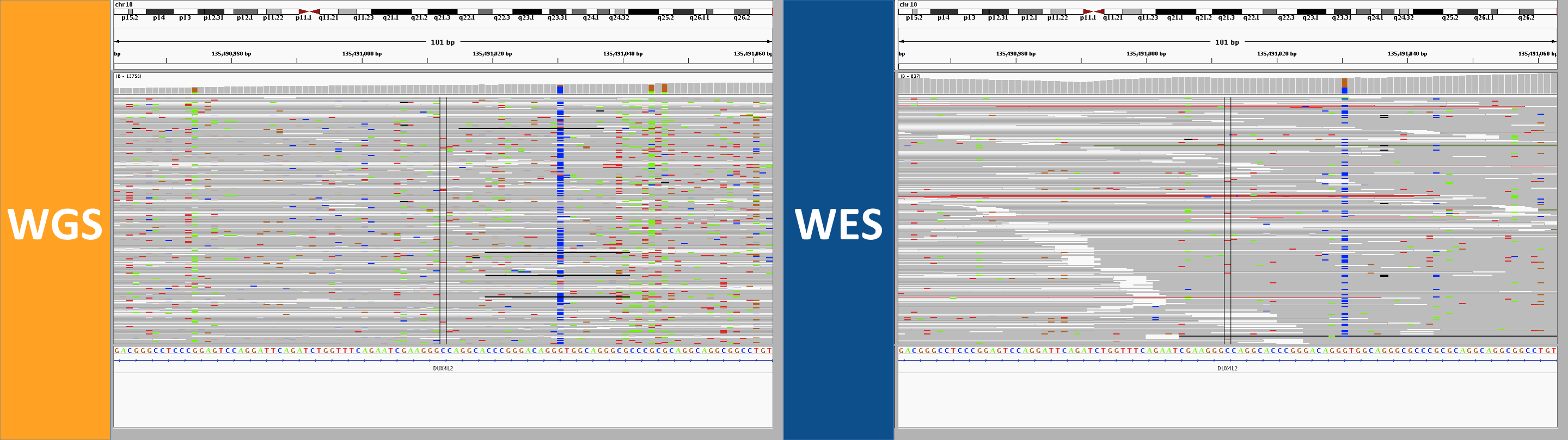
6. the curse of too much depth

This site in DUX4L2 is way out in the telomere at the end of the q end of chromosome 10. This is what’s known as a “collapsed repeat” – there are many near-identical tandem copies of this sequence in the human genome, but only one copy of the repeat is present in the reference genome. As a result there are a ton of reads here. The depth bar in the WGS screenshot goes up to 13,756 and in WES it goes to 837. While there is clearly a lot going on here, I’d say to be safe one might want to avoid calling any SNPs at all in this region. In WGS, however, several SNPs were called in this region. In WES, a different set of not-very-credible SNPs was called in this region, though in WES, most of them were filtered, whereas in WGS, they mysteriously achieved PASS scores. If you hover over the depth barplot for any one base, you’ll see they all have a mix of different bases:
This seemed to occur at sites with a massive amount of depth, yet the allelic depth reported by HaplotypeCaller was actually very low – in the individual in the above screenshot, the AD was listed as 2,1. This relates to the next category.
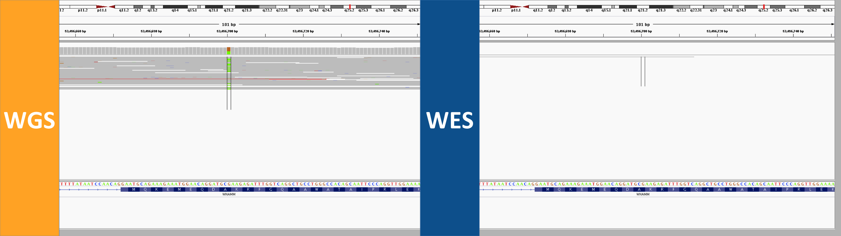
7. genotype calls without obvious read support

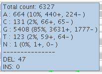
A surprisingly common category in the screenshots I looked at was cases where the reads appeared to provide no support whatsoever for the variant that was called. In WGS, a GGT>G deletion was called, and in WES it wasn’t called, but no reads in either dataset seemed to support the variant. On further inspection, the call in WGS was made with AD 6,0 and GQ 41.
Now, HaplotypeCaller does perform local realignment at complex sites, with the result that sometimes an IGV screenshot may not reflect the alignment on which the calls were based. However, in the example above, HaplotypeCaller recorded 0 alt alleles, so that can’t explain this call. One caveat for the analysis here is that the variant calls I’m analyzing were performed on a now-outdated version of GATK HaplotypeCaller in 2013 and so may reflect bugs that have since been fixed.
Although calls like this with no read support are probably just technical errors, I added this category to the list to remind us that not all of the ~2000 WGS-only alleles and ~500 WES-only alleles reflect differences in sequencing technology – some probably just reflect random error.
summary
Here I’ve compared WGS and WES data for the same 11 individuals. The libraries differ in depth, read length and PCR amplification in addition to exome capture, so the comparison will reflect all of these differences. WGS was able to cover 98.4% of the exome at a “callable” depth and quality, while WES covered only 93.5% at the same threshold. This probably reflects the more uniform distribution of coverage in our WGS data due to lack of capture and lack of PCR amplification, as well as the superior mappability of the longer reads. Consistent with WGS covering an additional ~5% of the exome, about 5% of exonic alt allele calls in WGS calls were unique to WGS and were not called in WES. Only about 1% of WES reads were unique to WES. Manual examination of the sites that were discordantly genotyped by the two technologies revealed several explanations. WGS gave superior variant calls where its longer reads gave better mappability or spanned short tandem repeats, where its coverage was more uniform either in total depth or in distribution of the position of a variant within a read, and where it gave more even allelic balance in loci where a high density of SNPs may have interfered with exome capture. WES and WGS both gave spurious variant calls at sites of extraordinarily high depth, and many calls in both datastes were simply not supported by reads at all.


