This post summarizes our recent manuscript on the application of transcriptome sequencing (RNA-seq) to the diagnosis of patients with Mendelian diseases, and provides a practical walk-through of our framework, methods and the Github code accompanying the paper).

Why RNA-seq for genetic diagnosis?

The current rate of genetic diagnoses across a variety of Mendelian disorders is approximately 25-50%. This means that more than half the families that come into the clinic searching for a genetic cause for their disease fail to receive a diagnosis.

There are a variety of reasons current diagnostic rates for Mendelian disorders are far from perfect. In some cases, the pathogenic variants are in genes that have not yet been established in the literature to cause the particular disorder, and with a single case, there isn’t enough evidence to make the diagnosis. There may also be complex inheritance patterns, such as digenic causes, to disorders that we have so far been underpowered to uncover. In addition, there are some key classes of variants where improvements in methods are still needed, such as calling structural variants from exome data or somatic variant discovery.

However, perhaps the most common driver for missed diagnoses is our inability to successfully functionally interpret the variants we see in patient DNA. This is especially true for variants we identify in whole genome sequencing (WGS) since our understanding of the non-coding genome remains limited, and the sheer number of these variants is overwhelming: in the gnomAD WGS database, every European carries an average of 7,067 variants that are not found in anyone else. This means that even frequency filtering with gnomAD leaves us with too many candidate variants for which the functional impact is unknown.

This is where RNA-seq comes in. RNA-seq offers a layer of functional information on top of what we know from the genetic analysis, and can help us begin to interpret some of the variants we identify with exome or whole genome sequencing, or identify new variants that may elude these technologies.

In our project we set about using RNA-seq to improve the diagnosis of a cohort of patients with a variety of severe, undiagnosed muscle diseases. We set out to look for splicing defects, allele imbalance, expression outlier status and to do variant calling directly on RNA-seq data. Our goal was to identify variants that may not have been captured with DNA-sequencing or to identify non-coding variants with functional impact that we may not have been properly interpreted. In the end, we were able to genetically diagnose 17 out of 50 undiagnosed patients, primarily through discovery of splice aberrations.

Some considerations for study design

Before applying RNA-seq to cohorts of undiagnosed Mendelian disease patients there are some critical questions to inform study design including i. what tissue to sequence ii. how many patients and controls to begin with and iii. what protocol and read depth to use for patient RNA-seq.

Based on multi-tissue transcriptome studies like GTEx, it is becoming increasingly clear that gene expression and splicing profiles can vary widely between tissues. Therefore to identify aberrations in these profiles, it is ideal to go after the disease-relevant tissue.

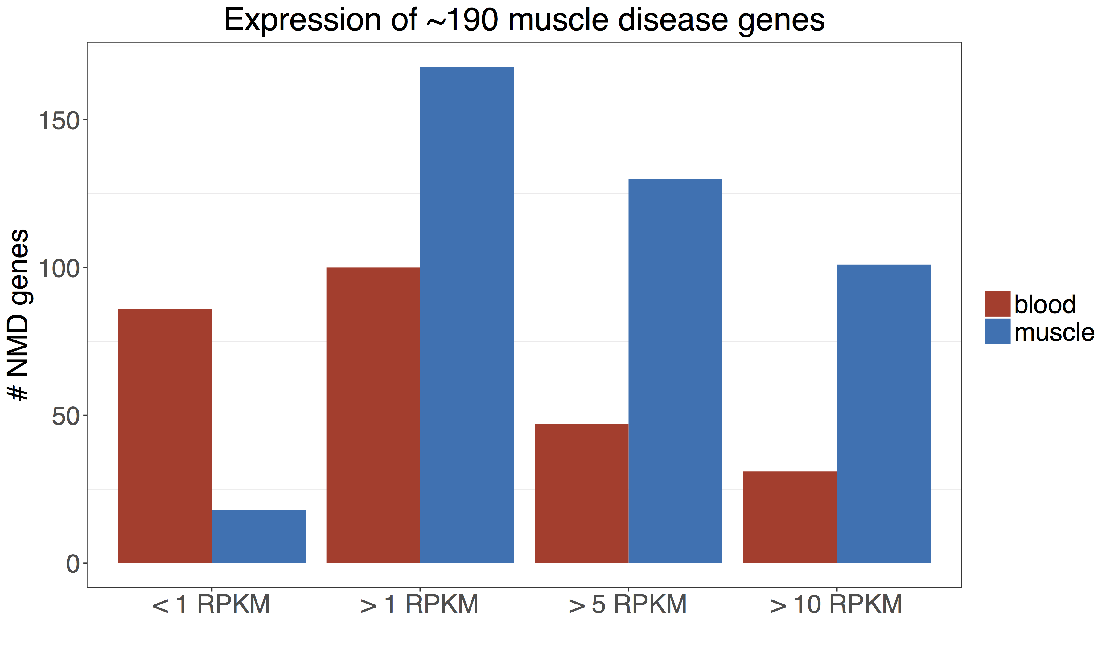
Consider the comparison below, showing the expression of ~190 Mendelian neuromuscular disease genes in GTEx blood and muscle, which suggests that almost half of these genes are below 1 RPKM in blood, a cutoff below which it is difficult to see enough reads in 50 million-paired end RNA-seq dataset to identify splice aberrations. This suggests that blood RNA-seq is a poor proxy for muscle for the purposes of diagnosis. We highly recommend performing a similar analysis based on your genes of interest in order to choose a proxy tissue for RNA-seq, if the disease-relevant tissue is unavailable.

Secondly, increasing the number of controls will increase your power to filter out non-deleterious junctions. We applied the framework laid out in the manuscript to identify “potentially pathogenic junctions” in 5 patients while increasing the number of GTEx controls. This shows that having few controls results in identifying more events that are seemingly unique to the patient. It also underlines the greater filtering power of having a specific gene list for the disorder of interest. Here, we recommend leveraging GTEx by choosing a proxy tissue represented in the dataset. If this is not possible, we would definitely recommend sequencing your own set of controls, and starting with at least ~20-30 samples.

Lastly, the protocol and read depth is dependent on whether you will be able to incorporate GTEx data into your analysis, in which case we recommend staying close to the GTEx protocol. Our patient samples were sequenced with 50 or 100 million paired-end reads and at a minimum, we recommend 50M paired-end reads. However, the precise impact of read depth will be dependent on the expression of your genes of interest, considering that expression of the disrupted gene in the patient may be decreased (for a gene in which recessive LOF mutations result in disease) and that larger genes will be more dramatically impacted by 3’ bias, which will lower your ability to have enough reads at the 3’ end of a gene to look for splice aberrations.

A reference panel of control tissue RNA-seq

Mendelian muscle disorders are a major disease focus in our lab. They are also a very practical place to test the value of RNA-seq for diagnosis: the collection and storage of frozen muscle biopsies is currently routine clinical practice for undiagnosed patients as they are used in protein studies, meaning that high-quality RNA from a disease-relevant tissue is available for a very large proportion of undiagnosed patients with these diseases.

One of the most powerful tools in Mendelian disease diagnosis are large-scale reference databases to look up the population frequency of a variant of interest (*cough gnomAD). This allows for filtering out events that are too common in the population to plausibly result in a Mendelian phenotype. We needed similar reference databases to filter events we identified in our patient muscle RNA-seq, so we turned to the Genotype Expression Project (GTEx) dataset, which is a large multi-tissue transcriptome sequencing effort that has sequenced across ~50 tissue types in ~600 individuals.  The GTEx inventory includes skeletal-muscle RNA-seq, so we integrated their data into our framework, which eliminated a need to obtain and sequence muscle tissue from healthy controls.

At the offset of the project, just over 400 skeletal-muscle RNA-seq samples were available from GTEx. We sub-selected 184 controls from GTEx that had high quality RNA-seq as well as phenotypic features that more closely matched our patient samples (see Methods section of the manuscript for more details).

Quality controlling patient RNA-seq data

We performed three main quality controls: i. technical QC ii. comparing gene expression profiles to GTEx samples to assess tissue quality iii. sample matching to ensure the source of RNA-seq was the proband for which we had prior information. This included fingerprinting comparison for WES/WGS /RNA-seq from the proband as well as checking to see if the sex entered for the patient validated in the RNA-seq, to ensure there were no sample mix-ups.

For technical QC, we obtained metrics by running RNA-seQC with gencode annotations obtained from the GTEx project.

For the tissue check, we used GTEx skeletal-muscle samples as well as tissues that potentially contaminate muscle biopsies such as skin or adipose to run principal component analysis (PCA) with our patient samples. Initially, we ran the PCA by using all genes, but now to QC each batch that comes in, we use tissue-preferentially expressed genes identified by GTEx, which produces similar results, but runs faster. A list of tissue-preferentially expressed genes are available in supplementary table S5 of this GTEx manuscript.

To validate the sex of the individual, we compared the average chrY and XIST expression and also clustered samples based on sex-preferentially expressed genes from the same GTEx paper as above.

There is example code and data in the Github page to check the clustering pattern of a randomly selected patient sample. You can see and run the code by cloning the repo https://github.com/berylc/MendelianRNA-seq.

in MendelianRNA-seq/QC 
For the muscle check:
$ Rscript MuscleCheck.R -patient_rpkm ../example/genes.rpkm.gct   
-out_file walkthrough.tissue 
 
and for the Sex Check:
$ Rscript SexCheck.R -patient_rpkm ../example/genes.rpkm.gct 
-out_file walkthrough.sex

Both commands create PDF files with plots for manual inspection and output text to indicate whether the samples cluster with muscle as well as their respective sex. In MuscleCheck.R, adding -writePCADat outputs the PC coordinates of all samples, in order to identify samples that may look like outliers by manual inspection.

Running these commands produces the plots below, which validate the RNA-seq sample is muscle and that the sample is male:

Default GTEx files to run this code for muscle RNA-seq are stored in Github. For the tissue check, you need an expression matrix of control tissues of interest and relevant tissue-preferentially expressed genes (ie. tissue_preferential_genes_fibs.msck.skn.adbp.txt and gtex_expression_tissue_preferential_fibs.msck.skn.adbp.txt in MendelianRNA-seq/data). For the sex check you need an expression matrix with sex-preferentially expressed genes (gtex_expression_sex_biased.txt). 

If you’d like to build a similar QC framework for a different set of tissues of interest, you can follow the code to create the GTEx expression matrices for sex and tissue-preferential genes:

in MendelianRNA-seq/data 
Get the required GTEx files:
$ wget -i gtex_file_urls
 
>Go through make_gtex_files.R and change the tissue names to create the files for your own tissues of interest.

Lastly, to ensure the sample for WES/WGS and RNA-seq are the same, we used PLINK to look at IBD estimates from ~5,800 common SNPs collated by Purcell et al. This code can be used to check relatedness within family WES/WGS/RNA-seq data as well.

in MendelianRNA-seq/QC 
-Note that to genotype RNA-seq files, you will need to split your BAMs first. You can do this by using GATK SplitNCigarReads. 
-You will also need to have GATK and PLINK installed, and point the scripts to a human genome reference fasta file.
 
1)Generate GVCFs from all bams you’re interested in checking
 
For a single BAM:
$ sh MakeGVCF.sh \
/path/to/gatk.jar \
/path/to/Homo_sapiens_assembly19.fasta \
/path/to/your.bam
 
2)Make a list of all output GVCFs and joint genotype for ~5,800k common SNPs
 
$ls -1 *vcf.gz > gvcfs.list
 
$ sh JointGenotype.sh \
/path/to/gatk.jar \
/path/to/Homo_sapiens_assembly19.fasta \
gvcfs.list
 
3)Make PLINK TFAM and TPED files for PLINK
 
$ zcat out.joint.vcf.gz | ./MakeTPED.pl > out.tped
$ zcat out.joint.vcf.gz | ./MakeTFAM.pl > out.tfam
 
4)Run PLINK
 
$ plink --noweb --tfile out --genome 
(you can add --min 0.1 which will set a threshold for the output)
 
>This will produce a plink.genome file, which has IBD values for your samples. We assessed the PI_HAT column to check relatedness. In our cohort the PI_HAT value for WES, WGS, and RNA-seq data from the same individuals ranged from 0.67-1.00 (mean = 0.9), compared to a range of 0-0.18 (mean= 0.001) for non-matching individuals.

(Re)processing patient and GTEx data

We downloaded and decrypted Tophat aligned BAM files from the GTEx dbGAP and realigned them with STAR 2-pass. We were specifically interested in unannotated splice events (ie. splice aberrations like exon skipping or intron inclusion) so we decided to align with STAR which we reasoned would be more sensitive to detect such events (relevant paper comparing several alignment methods found here).

In order to be as sensitive as possible to detect splice events with low-level read support, we concatenated 1st pass junctions identified across all samples and fed these junctions into the Star 2nd Pass alignment.  Please note that these steps are also laid out in the STAR manual for 2-pass alignment.

-You will need to have Picard and STAR installed for realignment
-You will also need to have created a STAR genome file for your RNA-seq protocol (see “Generating genome indices” in the STAR manual) 

In MendelianRNA-seq/Reprocessing
1)If you’re starting off with Tophat BAMs, turn them into fastqs
 
$ sh BamToFastq.sh /path/to/picard.jar /path/to/your.tophat.bam
 
2)Run STAR 1st pass to identify junctions
 
> 1stPassScript.sh is a wrapper around GeneralAlignment.sh which includes pre-specified alignment parameters for differing read lengths/sequencing types (stranded/unstranded, single-end/paired-end) etc. You can modify this script to specify the read length in your samples. It’s currently set up to align 76 bp unstranded paired-end RNA-seq (ie. GTEx RNA-seq)
 
$ sh ./1stPassScript.sh \
/path/to/your.tophat.bam \
/path/to/directory/containing/sample/fastq/directory \
/path/to/STAR/executable \ 
/path/to/STAR/genome
 
3)Concatenate all your junctions from the first pass alignment and filter the junctions to remove splice junctions on the mitochondrial genomes and unannotated junctions with less than 5 reads
 
$ cat *tab > all.SJout.tab
$ awk '$1!="MT"' all.SJout.tab | awk '$6~1' > final.filtered.SJout.tab
$ awk '$1!="MT"' all.SJout.tab | awk '$6~0' | awk 'int($7)>5' >> final.filtered.SJout.tab
 
4)Create a new STAR genome by aligning one sample. 
 
> This is the same as 1stPassScript.sh except now we add the junction file we created final.filtered.SJout.tab. This will align the one sample, and create a new genome file, which you will feed into the next step:
 
$ sh 2ndPassScript_CreateGenome.sh \
/path/to/your.tophat.bam \
/path/to/directory/containing/sample/fastq/ \
/path/to/STAR/executable \ 
/path/to/STAR/genome \
final.filtered.SJout.tab
 
5)Align all other samples using the new genome file created by the last step
 
$ sh 2ndPassScript_AllOthers.sh \
/path/to/your.tophat.bam \
/path/to/directory/containing/sample/fastq/ \
/path/to/STAR/executable 
/path/to/STAR/newly/created/STAR/genome
 
6)Mark Duplicates with Picard 
$ sh MarkDuplicates.sh /path/to/picard.jar /path/to/your.new.star.bam
 
>Note that if you have only a handful of samples, you can simply run (4) for all your samples, instead of doing a 2-step approach. This will create identical STAR genome for each samples, which you can delete.

Splice junction discovery and filtering

Our primary goal with splice junction analysis was to be able to identify splicing events that were found in one patient or groups of patients, and largely missing in GTEx controls. When we started the project, there were no easily adaptable tools that served this purpose. For example, DEXSEQ is a tool used for differential expression analysis, but it performs differential exon usage analysis to find global differences between experimental groups. Our goal was not to identify general exon-usage differences between diseased and healthy skeletal-muscle but to identify specific aberrations in specific individuals and look for the underlying genetic variants.

A year or so after we started the project, a software called Leafcutter was published, which can be used to identify sample-specific splice junctions. This paper used Leafcutter to identify sample-specific splice junctions, and was able to identify one sample with aberrant splicing out of 48 patients.

We developed our own pipeline that is composed of three steps i. Splice junction discovery from split reads ii. Normalization of read support for junctions based on local canonical splicing iii. Filtering splice junctions and spot-checking.

1- Splice junction discovery

We identified splice junctions supported by uniquely mapped split reads. This approach takes a gene annotation file and a list of BAM files as input, and identifies all the junctions in the samples.

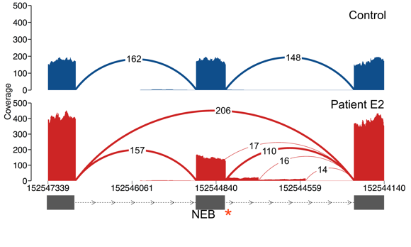
>We’ll run a mini-example of this using a subsetted bams from some patients in the manuscript (we use the subset so the data are unidentifiable) While the code is set up to run across many genes and bam files, we will run it on bams subsetted down to three exons in NEB, where one patient carries an essential splice site variant, to get a sense of how the scripts work. 

In MendelianRNA-seq/Analysis

$ sh SpliceJunctionDiscovery.sh ../example/example.gene.NEB.list ../example/patient.bam.list
 
$ head All.example.gene.NEB.list.splicing.txt
 
Gene Type Chrom Start End NTimesSeen NSamplesSeen Samples:NSeen
NEB protein_coding 2 152518855 152520062 1 1 Patient.D1.small:1
NEB protein_coding 2 152355006 152782552 1 1 Patient.D1.small:1
NEB protein_coding 2 152544892 152544894*1D17 1 1 Patient.E2.small:1
 
>The first three column names are self-explanatory; Start and End refer to the boundaries of the splice junction (ie Start and End are both exon-intron junctions), NTimesSeen is the total number of reads in the dataset that support that junction, NSamplesSeen is the number of samples the junction is seen in and the final column lays out the number of reads supporting the junction in each sample (sorted by read support so the sample with the highest read support is at the end). 
 
>Note that if you are doing this on bams you’ve aligned with a different method, you must assign unique mapping quality to be 60 (vs. the default 255). You can do this while you’re aligning with STAR using --outSAMmapqUnique 60 or you can use the GATK tool ReassignOneMappingQuality

1- Splice junction normalization

To identify potentially pathogenic splice evente, we may want to identify junctions that are unique to one individual. However, a pathogenic splice junction that only occurs in one sample in the whole dataset may still have read support in other samples, due to mapping noise. If a gene is highly expressed and/or if some samples have more reads sequenced, this may result in junctions that are present at very low levels in a sample to still to have high read support.

Here is a real example of a splice junction that is present in two individuals:

Gene	Splice junction	Total Read Support	Number of Samples	Sample : Read Support
TTN	2:179505357-179509275	78	2	Patient D10: 8, Patient N: 69

There are 69 reads in Patient N and 8 reads in Patient D10 that support this splice junction. It’s present in only two individuals and is in a known muscle disease gene, so it may be potentially interesting. From the read support data alone, it looks like it may be a real junction in Patient N and possibly mapping noise in Patient D10.

Here is a Sashimi plot of the local region in the two samples:

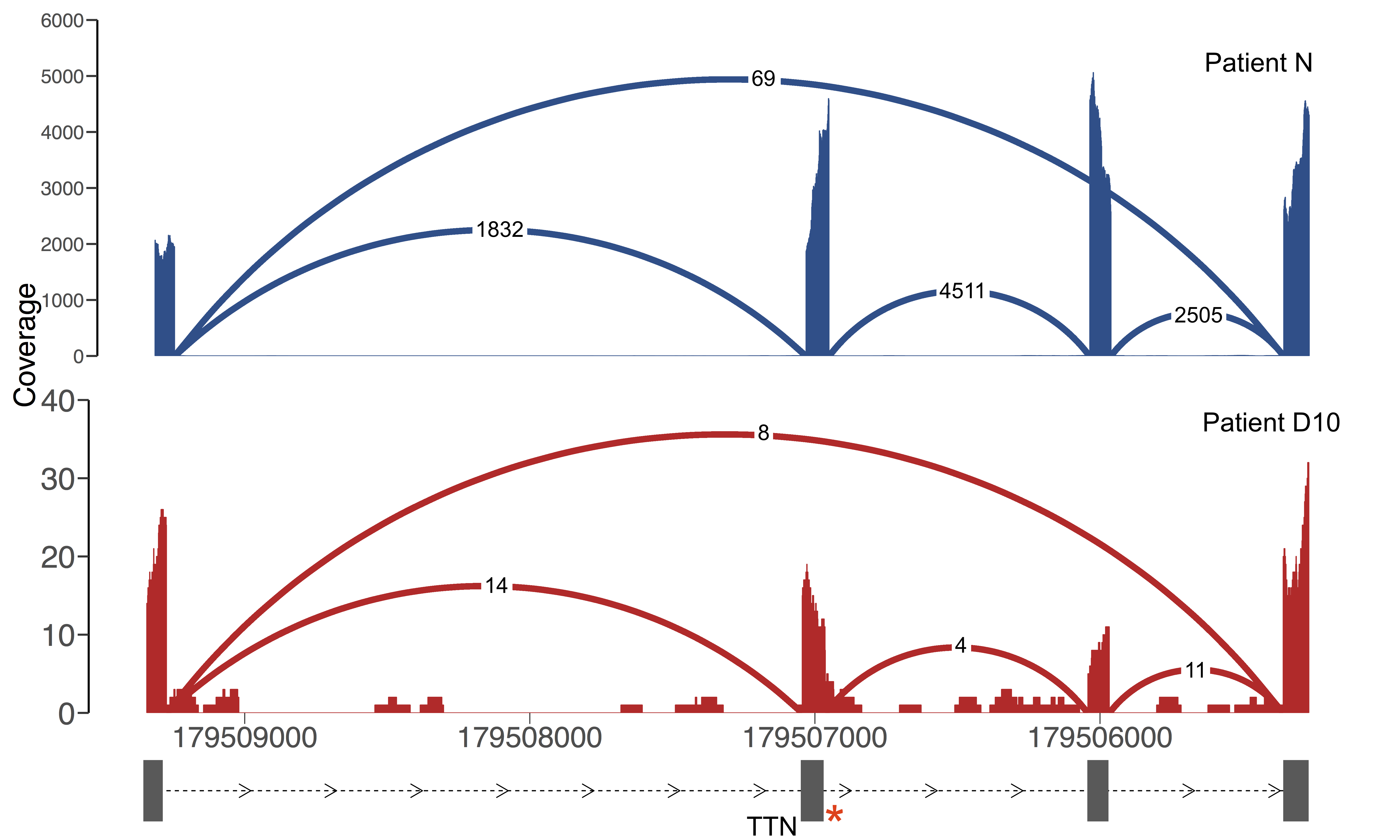
In fact, while there is higher read support for the junction in Patient N, the read support for the junction is only 1.5-4% of that of the canonical junctions. In contrast, the junction has 8 reads supporting it in Patient D10 but this constitutes ~50% of the read support for canonical reads, more in line with this being a heterozygous event. Patient D10 carries a heterozygous essential splice site variant (denoted by the red asterisk) which is causing exon skipping and this is more likely to be a low-level event or mapping noise in Patient N. The difference in read support between the two samples can be explained by the fact that Patient N was sequenced at 100M read depth compared to 50M in Patient D10, and that Patient D10 carries two LOF variants in TTN, which is decreasing expression of the gene.

In order to be able to access information on the relative support for a junction in the context of library size and gene expression, we normalize the splice junctions by the overlapping canonical junctions. This is explained in detail in the manuscript, specifically in Supplementary Figure 5. Note that you don’t have to run this normalization to be able to do filtering in the next step, but it does increase your filtering power.

in MendelianRNA-seq/Analysis 
$ python NormalizeSpliceJunctionValues.py -splice_file All.example.gene.NEB.list.splicing.txt --normalize > All.NEB.normalized.splicing.txt

This modifies the splice junction file in a few ways: it adds a column indicating the proportion of read support for the junction compared to the read support of the overlapping junction (ie. it would return  0.57 for Patient D10 and 0.04 for Patient N above). It also adds a column indicating whether both, one or neither exon-intron junctions are annotated. Both junctions being annotated can indicate a canonical splice event or exon skipping, one junction being annotated can indicate an exon extension, intronic splice-gain or exonic splice gain, and neither being annotated can indicate a structural variant

3- Splice junction filtering and visualization

The final step is to filter the file of junctions to identify potentially deleterious splice events. There are several different ways to do this filtering, such as looking for events that are only seen in one sample, with high read support. Alternatively you can look for splice junctions seen in many individuals, but only seen in one individual with read support higher than say, 20 reads (this would be one way to filter out mapping noise). You can also look for splice events that have over 100 reads supporting in the entire dataset, but seen in less than 5 individuals (to potentially identify groups of patients that have the splice event).  You can also utilize the normalization scheme developed above and only look for splice events that are seen at a level of 30% of the overlapping canonical junctions.

In other words, there are many way to look at the data to identify putatively pathogenic events, and the junctions you’d like to pull out will depend on your experimental design. Below we give a few examples that recover the exon skipping event in Patient E2.

in MendelianRNA-seq/Analysis 
$ python FilterSpliceJunctions.py -h
 
Should give you all the currently built in parameters to splice junction filtering along with their description

>Identify splice junctions that have at least 10 reads supporting the event:

$ python FilterSpliceJunctions.py -splice_file All.NEB.normalized.splicing.txt -n_read_support 10

>The coloring scheme will highlight the samples with the highest read support. This requires colorama and if you have Anaconda installed, it should run. If not, you can comment out “from colorama import.. “ at the beginning of the script. In this case, you can add the -print_simple argument, which will print without coloring. 

>Notice that the command above did not recover information about the normalized values of junction read support. This is set up so you can filter junctions without having to run NormalizeSpliceJunctionValues.py 

>To include the normalized values run: 

$ python FilterSpliceJunctions.py -splice_file All.NEB.normalized.splicing.txt -include_normalized 


>In some cases, you may want to filter out junctions where a samples have less than x number of reads. While in this case because we are only dealing with a 3-exon region, we don’t have much noise, generally this helps reduce the number of non-deleterious events you identify. 

$ python FilterSpliceJunctions.py -splice_file All.NEB.normalized.splicing.txt -n_read_support 10 -include_normalized -filter_n_reads 5 

> Notice that sample N27 only had 3 reads aligning to junction 2:152544910-152547241 (total read support for the junction : 493). When we filtered samples with less than 5 reads, this removed N27 from the line, and also decreased the number of samples the junction is seen in from 3 to 2, and subtracted the read support for the sample (total read support for the junction became 490). We usually only set filter_n_reads to 2 or 3, to filter out very low-level events. 

>Identify splice junctions where the highest normalized read support is seen in a specific sample: 

$ python FilterSpliceJunctions.py -splice_file All.NEB.normalized.splicing.txt -n_read_support 10 -include_normalized -sample_with_highest_normalized_read_support Patient.E2.small 

>Or simply identify junctions that are only seen in one sample 

$python FilterSpliceJunctions.py -splice_file All.NEB.normalized.splicing.txt -n_read_support 10 -include_normalized -n_samples 1 

> You can also add OMIM information to the junction file:  

$ python FilterSpliceJunctions.py -splice_file All.NEB.normalized.splicing.txt -n_read_support 10 -include_normalized -filter_n_reads 5 -add_OMIM 

> To only show junctions occurring in OMIM genes you can add -only_OMIM. You can also only show junctions in specific genes of interest by adding say, -genes NEB,TTN,CAPN3. 

In this example, searching for junctions that are present in one sample leads us to the essential splice site in this patient. In fact, all four splice junctions that we identify as only being present in Patient E2 are due to this single variant, which is abolishing splicing at the canonical junction, resulting in both exon skipping as well as splicing from intact motifs within the intron.

Future plans

We hope that the steps described above will give those interested a start to applying splice junction analysis to their own patient cohorts.

However, what’s needed long-term is a fully functional (and largely automated) tool for RNA-seq-guided diagnosis that is usable by non-bioinformaticians. To that end, we are currently working on the development of a web-based tool to perform such analyses and visualize splice junctions, without requiring any command-line experience. We’ll announce that tool here as soon as it’s ready.

We are also continuing to apply RNA-seq as part of the Broad Center for Mendelian Disease Genetics, with a focus on novel disease gene discovery. In this effort, we have expanded RNA-seq out to other areas and tissue types such kidney biopsy RNA-seq from patients with Mendelian forms of kidney disease. We are also interested in exploring the use of proxy tissues and are performing fibroblast RNA-seq for a variety of Mendelian disorders. If you are interested in submitting genetically undiagnosed patients for RNA-seq as part of the CMG, please visit https://cmg.broadinstitute.org/Apply.